---
title: "QFeatures in a nutshell"
author:
- name: Laurent Gatto
- name: Christophe Vanderaa
output:
BiocStyle::html_document:
self_contained: yes
toc: true
toc_float: true
toc_depth: 2
code_folding: show
bibliography: scp.bib
date: "`r BiocStyle::doc_date()`"
package: "`r BiocStyle::pkg_ver('scp')`"
vignette: >
%\VignetteIndexEntry{QFeatures in a nutshell}
%\VignetteEngine{knitr::rmarkdown}
%\VignetteEncoding{UTF-8}
---
```{r setup, include = FALSE}
knitr::opts_chunk$set(
collapse = TRUE,
comment = "#>",
crop = NULL
## cf https://stat.ethz.ch/pipermail/bioc-devel/2020-April/016656.html
)
```
This vignette briefly recaps the main concepts of `QFeatures` on which
`scp` relies. More in depth information is to be found in the
`QFeatures` [vignettes](https://rformassspectrometry.github.io/QFeatures/articles/QFeatures.html).
# The `QFeatures` class
The `QFeatures` class (@Gatto2023-ry) is based on the
`MultiAssayExperiment` class that holds a collection of
`SummarizedExperiment` (or other classes that inherits from it)
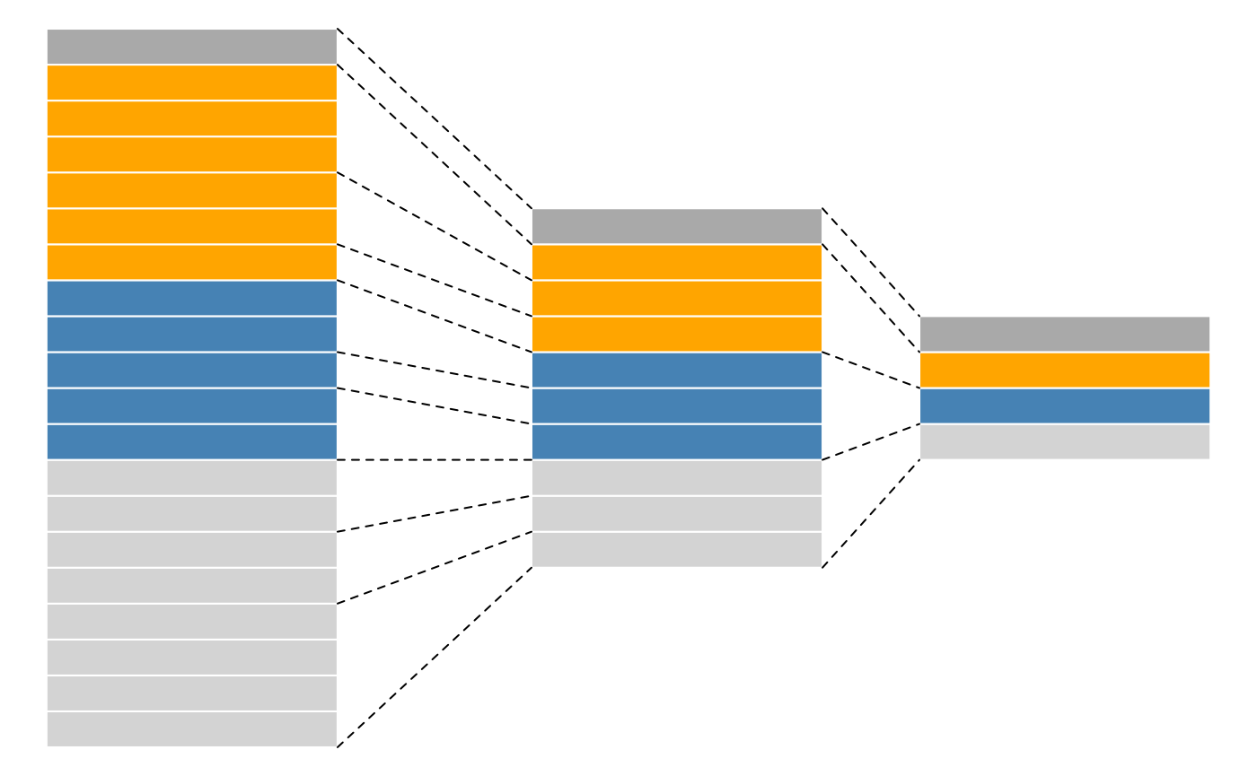
objects termed **assays**. The assays in a `QFeatures` object have a
hierarchical relation: proteins are composed of peptides, themselves
produced by spectra, as depicted in figure below.
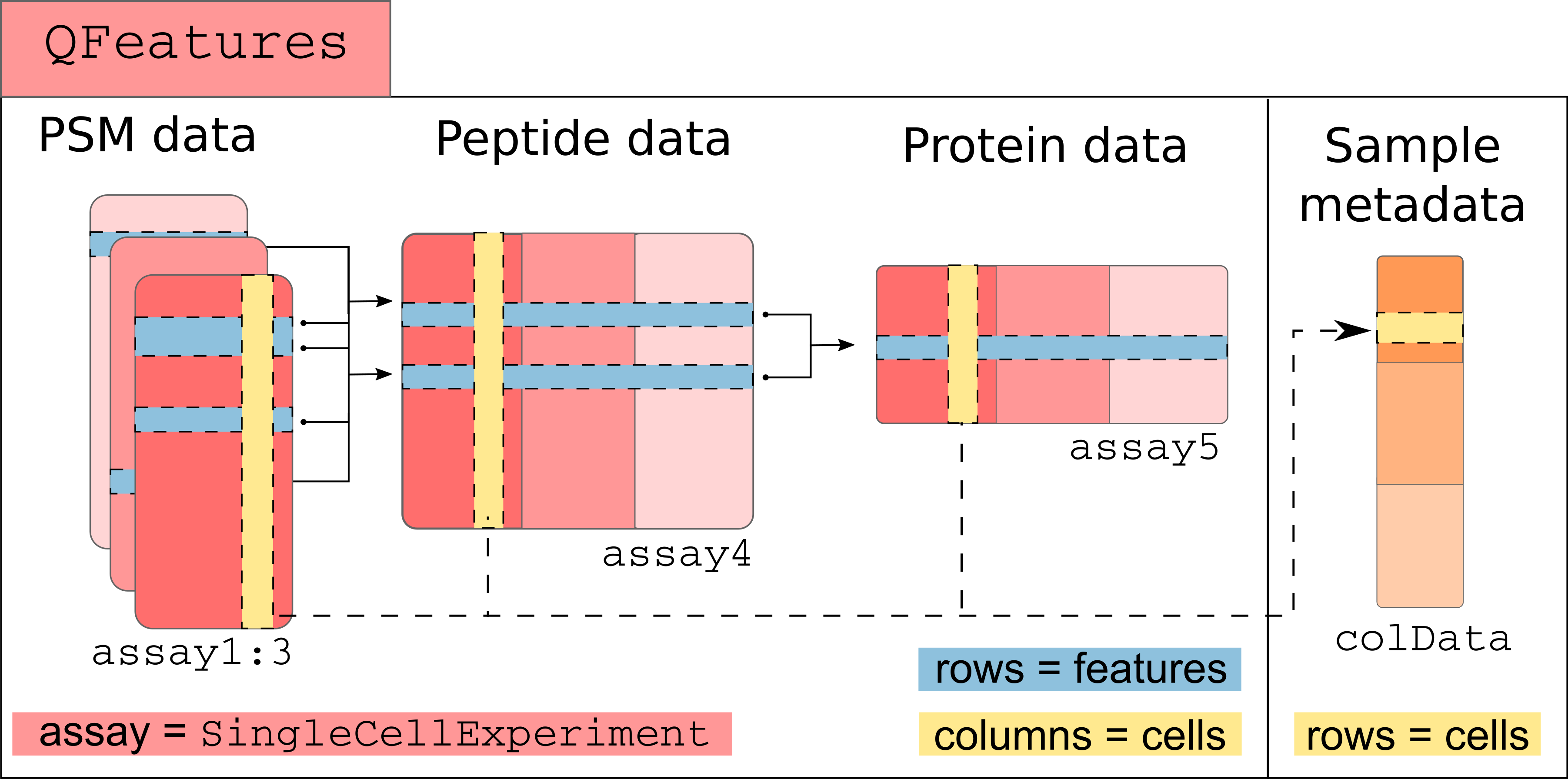
A more technical representation is shown below, highlighting that each
assay is a `SummarizedExperiment` (containing the quantitative data,
row and column annotations for each individual assay), as well as a
global sample annotation table, that annotates cells across all
assays.
Those links are stored as part as the `QFeatures` object and connect
the assays together. We load an example dataset from the `scp` package
that is formatted as an `QFeatures` object and plot those connection.
```{r hierarchy, message = FALSE, out.width = "600px"}
library(scp)
data("scp1")
plot(scp1)
```
# Accessing the data
The `QFeatures` class contains all the available and metadata. We here
show how to retrieve those different pieces of information.
## Quantitative data
The quantitative data, stored as matrix-like objects, can be accessed
using the `assay` function. For example, we here extract the
quantitative data for the first MS batch (and show a subset of it):
```{r assay_data}
assay(scp1, "190321S_LCA10_X_FP97AG")[1:5, ]
```
Note that you can retrieve the list of available assays in a
`QFeatures` object using the `names()` function.
```{r names}
names(scp1)
```
## Feature metadata
For each individual assay, there is feature metadata available. We
extract the list of metadata tables by using `rowData()` on the
`QFeatures` object.
```{r rowData}
rowData(scp1)
rowData(scp1)[["proteins"]]
```
You can also retrieve the names of each `rowData` column for all
assays with `rowDataNames`.
```{r rowDataNames}
rowDataNames(scp1)
```
You can also get the `rowData` from different assays in a single table
using the `rbindRowData` function. It will keep the common `rowData`
variables to all selected assays (provided through `i`).
```{r rbindRowData}
rbindRowData(scp1, i = 1:5)
```
## Sample metadata
The sample metadata is retrieved using `colData` on the `QFeatures`
object.
```{r colData}
colData(scp1)
```
Note that you can easily access a `colData` column using the `$`
operator. See here how we extract the sample types from the `colData`.
```{r colData_dollar}
scp1$SampleType
```
# Subsetting the data
There are three dimensions we want to subset for:
- Assays
- Samples
- Features
Therefore, `QFeatures` support a three-index subsetting. This is
performed through the simple bracket method `[feature, sample, assay]`.
## Subset assays
Suppose that we want to focus only on the first MS batch
(`190321S_LCA10_X_FP97AG`) for separate processing of the data.
Subsetting the `QFeatures` object for that assay is simply:
```{r subset_assay}
scp1[, , "190321S_LCA10_X_FP97AG"]
```
An alternative that results in exactly the same output is using the
`subsetByAssay` method.
```{r, subsetByAssay}
subsetByAssay(scp1, "190321S_LCA10_X_FP97AG")
```
## Subset samples
Subsetting samples is often performed after sample QC where we want to
keep only quality samples and sample of interest. In our example, the
different samples are either technical controls or single-cells
(macrophages and monocytes). Suppose we are only interested in
macrophages, we can subset the data as follows:
```{r, subset_samples}
scp1[, scp1$SampleType == "Macrophage", ]
```
An alternative that results in exactly the same output is using the
`subsetByColData` method.
```{r, subsetByColData}
subsetByColData(scp1, scp1$SampleType == "Macrophage")
```
## Subset features
Subsetting for features does more than simply subsetting for the
features of interest, it will also take the features that are linked
to that feature. Here is an example, suppose we are interested in the
`Q02878` protein.
```{r subset_features}
scp1["Q02878", , ]
```
You can see it indeed retrieved that protein from the `proteins` assay,
but it also retrieved 11 associated peptides in the `peptides` assay
and 19 associated PSMs in 2 different MS runs.
An alternative that results in exactly the same output is using the
`subsetByColData` method.
```{r, subsetByFeature}
subsetByFeature(scp1, "Q02878")
```
You can also subset features based on the `rowData`. This is performed
by `filterFeatures`. For example, we want to remove features that are
associated to reverse sequence hits.
```{r, filterFeatures}
filterFeatures(scp1, ~ Reverse != "+")
```
Note however that if an assay is missing the variable that is used to
filter the data (in this case the `proteins` assay), then all features
for that assay are removed.
You can also subset the data based on the feature missingness using
`filterNA`. In this example, we filter out proteins with more than
70 \% missing data.
```{r, filterNA}
filterNA(scp1, i = "proteins", pNA = 0.7)
```
# Common processing steps
We here provide a list of common processing steps that are encountered
in single-cell proteomics data processing and that are already
available in the `QFeatures` package.
All functions below require the user to select one or more assays from
the `QFeatures` object. This is passed through the `i` argument. Note
that some datasets may contain hundreds of assays and providing the
assay selection manually can become cumbersome. We therefore suggest
the user to use regular expression (aka regex) to chose from the
`names()` of the `QFeautres` object. A detailed cheatsheet about regex
in R can be found
[here](https://rstudio-pubs-static.s3.amazonaws.com/74603_76cd14d5983f47408fdf0b323550b846.html).
## Missing data assignment
It often occurs that in MS experiements, 0 values are not true zeros
but rather signal that is too weak to be detected. Therefore, it is
advised to consider 0 values as missing data (`NA`). You can use
`zeroIsNa` to automatically convert 0 values to `NA` in assays of
interest. For instance, we here replace missing data in the `peptides`
assay.
```{r, zeroIsNA}
table(assay(scp1, "peptides") == 0)
scp1 <-zeroIsNA(scp1, "peptides")
table(assay(scp1, "peptides") == 0)
```
## Feature aggregation
Shotgun proteomics analyses, bulk as well as single-cell, acquire and
quantify peptides. However, biological inference is often performed at
protein level. Protein quantitations can be estimated through feature
aggregation. This is performed by `aggregateFeatures`, a function that
takes an assay from the `Qfeatures` object and that aggregates its
features with respect to a grouping variable in the `rowData` (`fcol`)
and an aggregation function.
```{r aggregateFeatures}
aggregateFeatures(scp1, i = "190321S_LCA10_X_FP97AG", fcol = "protein",
name = "190321S_LCA10_X_FP97AG_aggr",
fun = MsCoreUtils::robustSummary)
```
You can see that the aggregated function is added as a new assay to
the `QFeatures` object. Note also that, under the hood,
`aggregateFeatures` keeps track of the relationship between the
features of the newly aggregated assay and its parent.
## Normalization
An ubiquituous step that is performed in biological data analysis is
normalization that is meant to remove undesired variability and to
make different samples comparable. The `normalize` function offers an
interface to a wide variety of normalization methods. See
`?MsCoreUtils::normalize_matrix` for more details about the available
normalization methods. Below, we normalize the samples so that they
are mean centered.
```{r normalize}
normalize(scp1, "proteins", method = "center.mean",
name = "proteins_mcenter")
```
Other custom normalization can be applied using the `sweep` method,
where normalization factors have to be supplied manually. As an example,
we here normalize the samples using a scaled size factor.
```{r sweep}
sf <- colSums(assay(scp1, "proteins"), na.rm = TRUE) / 1E4
sweep(scp1, i = "proteins",
MARGIN = 2, ## 1 = by feature; 2 = by sample
STATS = sf, FUN = "/",
name = "proteins_sf")
```
## Log transformation
The `QFeatures` package also provide the `logTransform` function to
facilitate the transformation of the quantitative data. We here show
its usage by transforming the protein data using a base 2 logarithm
with a pseudo-count of one.
```{r logTransform}
logTransform(scp1, i = "proteins", base = 2, pc = 1,
name = "proteins_log")
```
## Imputation
Finally, `QFeatures` offers an interface to a wide variety of
imputation methods to replace missing data by estimated values. The
list of available methods is given by `?MsCoreUtils::impute_matrix`.
We demonstrate the use of this function by replacing missing data
using KNN imputation.
```{r impute}
anyNA(assay(scp1, "proteins"))
scp1 <- impute(scp1, i = "proteins", method ="knn", k = 3)
anyNA(assay(scp1, "proteins"))
```
# Data visualization
Visualization of the feature and sample metadata is rather
straightforward since those are stored as tables (see section
*Accessing the data*). From those tables, any visualization tool can
be applied. Note however that using `ggplot2` require `data.frame`s or
`tibble`s but `rowData` and `colData` are stored as `DFrames` objects.
You can easily convert one data format to another. For example, we
plot the parental ion fraction (measure of spectral purity) for each
of the three MS batches.
```{r vis1, message = FALSE, fig.width = 6.5}
rd <- rbindRowData(scp1, i = 1:3)
library("ggplot2")
ggplot(data.frame(rd)) +
aes(y = PIF,
x = assay) +
geom_boxplot()
```
Combining the metadata and the quantitative data is more challenging
since the risk of data mismatch is increased. The `QFeatures` package
therefore provides th `longFormat` function to transform a `QFeatures`
object in a long `DFrame` table. For instance, we plot the
quantitative data distribution for the first assay according to the
acquisition channel index and colour with respect to the sample type.
Both pieces of information are taken from the `colData`, so we provide
them as `colvars`.
```{r longFormat}
lf <- longFormat(scp1[, , 1],
colvars = c("SampleType", "Channel"))
ggplot(data.frame(lf)) +
aes(x = Channel,
y = value,
colour = SampleType) +
geom_boxplot()
```
A more in-depth tutorial about data visualization from a `QFeatures`
object is provided in the `QFeautres` visualization
[vignette](https://rformassspectrometry.github.io/QFeatures/articles/Visualization.html).
# Session information {-}
```{r setup2, include = FALSE}
knitr::opts_chunk$set(
collapse = TRUE,
comment = "",
crop = NULL
)
```
```{r sessioninfo, echo=FALSE}
sessionInfo()
```
# License {-}
This vignette is distributed under a
[CC BY-SA license](https://creativecommons.org/licenses/by-sa/2.0/)
license.
# Reference {-}